Autoencoders Data Compression With PyTorch

Data Compression Using Autoencoders on Fashion MNIST

Project Overview

This project implements an autoencoder neural network in PyTorch to compress and reconstruct images from the Fashion MNIST dataset. Autoencoders are unsupervised learning models that learn efficient data representations (encodings) by compressing the input into a latent space and then reconstructing it.

What is an Autoencoder?

An autoencoder consists of two main components:

1. Encoder: Compresses the input into a lower-dimensional representation (latent space)
2. Decoder: Reconstructs the input from the compressed representation

The model is trained to minimize the difference between the original input and its reconstruction, forcing it to learn the most important features of the data.

• Dataset: Fashion MNIST (28×28 grayscale images of clothing items)
• Compression: 784 (28×28) → 64 dimensions (91.8% reduction)
• Evaluation: Uses both MSE (pixel-level error) and SSIM (perceptual quality)
• Training: Implements early stopping to prevent overfitting

1. Data Loading and Preparation

# Define image transformation (convert to tensor)
transform = transforms.Compose([transforms.ToTensor()])

# Download and load Fashion MNIST dataset
train_dataset = datasets.FashionMNIST(root='./data', train=True, download=True, transform=transform)
test_dataset = datasets.FashionMNIST(root='./data', train=False, download=True, transform=transform)

# Create data loaders for batch processing
train_loader = DataLoader(train_dataset, batch_size=128, shuffle=True)
test_loader = DataLoader(test_dataset, batch_size=128, shuffle=False)

Data Loading Explained

The code above performs several important steps:

1. Transformation: Converts images to PyTorch tensors (required for neural network processing)
2. Dataset Loading: Downloads Fashion MNIST if not already available locally
3. Data Loaders: Creates iterable objects that:
   • Handle batching (128 images at a time)
   • Shuffle training data (important for proper learning)
   • Provide efficient data loading during training

Each image is 28×28 pixels with single channel (grayscale), so each image is represented as a 1×28×28 tensor.

2. Autoencoder Architecture

class Autoencoder(nn.Module):
    def __init__(self):
        super().__init__()
        # Encoder: Compresses the input to a latent space representation
        self.encoder = nn.Sequential(
            nn.Flatten(),                     # Convert 28x28 image to 784-dim vector
            nn.Linear(784, 256),               # First compression layer
            nn.ReLU(),                         # Non-linearity for learning complex patterns
            nn.Linear(256, 64),                # Bottleneck layer (64-dimensional latent space)
            nn.ReLU()
        )
        
        # Decoder: Reconstructs the input from the latent space
        self.decoder = nn.Sequential(
            nn.Linear(64, 256),                # First expansion layer
            nn.ReLU(),
            nn.Linear(256, 784),               # Final layer reconstructs original dimensions
            nn.Sigmoid(),                      # Output values between 0 and 1 (like input)
            nn.Unflatten(1, (1, 28, 28))      # Reshape to original image dimensions

    def forward(self, x):
        # Pass input through encoder then decoder
        return self.decoder(self.encoder(x))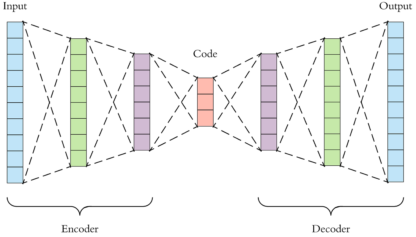

Visualization of autoencoder architecture (source: Medium)

Architecture Details

The autoencoder follows this dimensional transformation:

• Input: 1×28×28 image (784 pixels when flattened)
• Encoder:
  • 784 → 256 (first hidden layer)
  • 256 → 64 (bottleneck/latent space)
• Decoder:
  • 64 → 256 (mirrors encoder)
  • 256 → 784 (back to original size)

Key Components:

1. Flatten/Unflatten: Converts between image and vector representations
2. ReLU Activation: Introduces non-linearity for learning complex patterns
3. Sigmoid Output: Ensures output values match input range (0-1)
4. Bottleneck (64 units): Forces the network to learn compressed representations

Design Choice: The bottleneck size (64) represents a trade-off between compression and reconstruction quality. Smaller sizes increase compression but may lose important features.

3. Early Stopping Implementation

class EarlyStopping:
    def __init__(self, patience=5, min_delta=0.001):
        """
        Args:
            patience: Number of epochs to wait before stopping when loss isn't improving
            min_delta: Minimum change in loss to qualify as an improvement
        """
        self.patience = patience
        self.min_delta = min_delta
        self.counter = 0
        self.best_loss = None

    def __call__(self, val_loss):
        """
        Check if training should stop based on current validation loss
        
        Returns:
            True if training should stop, False otherwise
        """
        if self.best_loss is None:
            # First validation check
            self.best_loss = val_loss
            return False
        elif val_loss < self.best_loss - self.min_delta:
            # Significant improvement - reset counter
            self.best_loss = val_loss
            self.counter = 0
            return False
        else:
            # No improvement - increment counter
            self.counter += 1
            return self.counter >= self.patience

Early Stopping Mechanism

Early stopping prevents overfitting by monitoring the validation loss and stopping training when the model stops improving.

How it works:

1. Initialization: Sets up patience (number of allowed non-improving epochs) and minimum delta (required improvement threshold)
2. Tracking: Maintains the best observed loss value and a counter of non-improving epochs
3. Decision Logic:
   • If loss improves by at least min_delta, reset counter
   • If no significant improvement, increment counter
   • Stop when counter reaches patience value

Why use early stopping? It helps prevent overfitting while also saving computation time by stopping training once the model has converged.

4. Model Training Process

# Initialize model, loss function, and optimizer
model = Autoencoder()
criterion = nn.MSELoss()  # Mean Squared Error loss
optimizer = optim.Adam(model.parameters(), lr=1e-3)  # Adaptive learning rate
early_stopping = EarlyStopping(patience=5)

# Training loop
for epoch in range(50):  # Maximum 50 epochs
    model.train()  # Set model to training mode
    total_loss = 0
    
    # Batch processing
    for inputs, _ in train_loader:  # Ignore labels (unsupervised)
        # Forward pass
        optimizer.zero_grad()  # Clear previous gradients
        outputs = model(inputs)  # Generate reconstructions
        loss = criterion(outputs, inputs)  # Compare to original
        
        # Backward pass and optimization
        loss.backward()  # Compute gradients
        optimizer.step()  # Update weights
        total_loss += loss.item()  # Accumulate loss
    
    # Epoch statistics
    avg_loss = total_loss / len(train_loader)
    print(f"Epoch {epoch+1}, Loss: {avg_loss:.4f}")
    
    # Early stopping check
    if early_stopping(avg_loss):
        print("Early stopping triggered.")
        break

Training Breakdown

The training process follows these steps for each epoch:

1. Initialization

• Model: Creates autoencoder instance
• Loss Function: MSE measures pixel-wise difference between original and reconstructed images
• Optimizer: Adam adapts learning rates for each parameter

2. Training Loop

1. Batch Processing: Processes 128 images at a time
2. Forward Pass:
   • Clears old gradients (zero_grad)
   • Generates reconstructions
   • Calculates reconstruction error
3. Backward Pass:
   • Computes gradients (backward)
   • Updates weights (step)

3. Early Stopping Check

After each epoch, checks if loss has improved sufficiently to continue training.

Training Dynamics: The loss should decrease rapidly at first, then more slowly as the model converges. Early stopping typically triggers after 15-30 epochs for this problem.

5. SSIM Evaluation & Visualization

def compute_ssim(img1, img2, sigma=1.5):
    """
    Compute Structural Similarity Index (SSIM) between two images.
    SSIM measures perceptual similarity (range: -1 to 1, with 1 being identical)
    """
    # Convert tensors to numpy arrays
    img1 = img1.detach().numpy().squeeze()
    img2 = img2.detach().numpy().squeeze()
    
    # Parameters for SSIM calculation
    win_size = 3
    k1, k2 = 0.01, 0.03
    L = 1  # Dynamic range of pixels
    
    # Calculate means, variances, and covariance
    mu1 = gaussian_filter(img1, sigma)
    mu2 = gaussian_filter(img2, sigma)
    # ... (full SSIM calculation continues)
    
    return np.mean(ssim_map)

def evaluate(model, test_loader):
    """Evaluate model on test set and visualize results"""
    model.eval()  # Set to evaluation mode
    with torch.no_grad():  # Disable gradient calculation
        for inputs, _ in test_loader:
            outputs = model(inputs)
            
            # Calculate metrics
            mse = F.mse_loss(outputs, inputs).item()
            ssim = compute_ssim(outputs, inputs)
            
            # Visualize first 5 samples
            fig, axes = plt.subplots(2, 5, figsize=(15, 6))
            for i in range(5):
                axes[0,i].imshow(inputs[i].squeeze(), cmap='gray')
                axes[1,i].imshow(outputs[i].squeeze(), cmap='gray')
                axes[0,i].set_title(f"Original {i+1}")
                axes[1,i].set_title(f"Recon. {i+1}\nSSIM: {ssim[i]:.3f}")
            plt.show()
            break  # Only evaluate first batch

Example of original (top) and reconstructed (bottom) images with SSIM scores

Evaluation Metrics

We use two complementary metrics to assess reconstruction quality:

1. Mean Squared Error (MSE)

• Measures average squared difference between pixels
• Simple to compute but doesn't always match human perception
• Formula: MSE = 1/n Σ (original - reconstructed)²

2. Structural Similarity Index (SSIM)

• Perceptual metric that considers luminance, contrast, and structure
• Range: -1 (completely different) to 1 (identical)
• Generally > 0.7 indicates good reconstruction
• More computationally intensive than MSE

Why both metrics? MSE gives a global error measure while SSIM better captures perceptual quality. They often correlate but can disagree in some cases.

Key Learnings and Insights

• Dimensionality Reduction: The autoencoder successfully compresses 784-dimensional images to just 64 dimensions (91.8% reduction) while preserving most visual information.
• Feature Learning: The bottleneck forces the network to learn the most important features of clothing items (edges, shapes, textures) rather than memorizing pixels.
• Evaluation Metrics: SSIM (Structural Similarity Index) often correlates better with human perception of image quality than MSE, especially for images with subtle differences.
• Training Optimization: Early stopping effectively prevents overfitting while saving computation time, typically stopping training after 15-30 epochs.
• Architecture Choices: The symmetric encoder-decoder structure with ReLU activations and a sigmoid output provides good reconstruction quality while maintaining stable training.

Potential Improvements

This basic autoencoder could be enhanced with:

1. Convolutional Layers: Replace fully-connected layers with CNNs to better capture spatial relationships
2. Variational Autoencoder: Add probabilistic sampling for generative capabilities
3. Denoising: Train with noisy inputs to improve robustness
4. Different Bottleneck Sizes: Experiment with compression ratios (e.g., 32 or 128 units)